Lecture 02: Text Classification – BoW Representation and Logistic Regression
This lecture introduces the fundamental concepts of text classification, a core task in Natural Language Processing (NLP). We will cover the definition of text classification, how to represent text numerically, and a classic machine learning model for this task: logistic regression.
Section I: Text Classification: Definition
An example of text classification is sentiment classification, where texts from various sources such as movie reviews, product reviews, and customer feedback are categorized based on sentiment.

Another common application is news classification, which involves categorizing news articles into different topics, as shown in the following screenshot.

For those interested in a hands-on experience, an interactive text classifier demo is available on Hugging Face. Note that, the backend system of this classifier is LLMs, which will be explained in a later lecture.

In a text classification task, the input is a text denoted by \( x \), which can be a document, paragraph, sentence, or even a single word. The output is a classification label \( y \) from a pre-defined set. For example, in sentiment classification, the label set could be {positive, negative} or {1, 0}.
I.1 A Simple Demo Code
Building a text classifier is no longer a challenging task. The following Python code with the APIs from scikit-learn is good enough to demonstrate how to build a simple text classifier.
# 1. Convert text into numeric vectors
vectorizer = CountVectorizer()
X_train = vectorizer.fit_transform(X_train)
X_test = vectorizer.transform(X_test)

# 2. Initialize and train a classifier
model = LogisticRegression()
model.fit(X_train, y_train)

# 3. Make predictions and report prediction accuracy
y_pred = model.predict(X_test)
print(accuracy_score(y_test, y_pred))
This demo is available in the first section of this Google Colab note.
I.2 A Formal Formulation
The basic pipeline of text classification consists of two main stages. First, texts and labels are converted into numeric representations. Second, a classifier is built to capture the relationship between these texts and their corresponding labels.

There are several methods for creating numeric representations of texts. The bag-of-words representation, which converts texts into sparse representations, will be explained in this lecture. Other methods, such as word embeddings and representations from Large Language Models (LLMs), will be covered in future lectures.
A classifier can be formulated as a model of the conditional probability of a label \( y \) given a text \( x \), written as \( P(Y=y\mid X=x) \) or simply \( P(y\mid x) \). In this formulation, both \( x \) and \( y \) are the numeric vectors from the first stage.
Prediction is performed by finding the label \( \hat{y} \) that maximizes this conditional probability, as shown in the equation:
\[\hat{y}=\arg\max_{y\in\mathcal{Y}}P(y\mid x)\]where $\arg\max_y$ is to find a value of $y$ from $\mathcal{Y}$ that can maximizes the conditional probability $P(y\mid x)$.
There are several ways to build text classifiers, including logistic regression, feed-forward neural networks, and large language models. Other classifiers, such as Bayes classifiers, support vector machines, and convolutional neural networks, can also be used.
Section II: Bag-of-Words Representations
Let’s consider two example texts to illustrate the bag-of-words representation:
- Text 1: I love coffee.
- Text 2: I don’t like tea.
The first step is tokenization, where a text is converted into a collection of tokens. If we use punctuation and white space as boundaries for tokenization, the tokenized texts are I, love, coffee for the first text, and I, don, t, like, tea for the second.
Different tokenization methods can be used. For the input I don't like tea., white-space based tokenization would produce ["I", "don't" "like", "tea."], while a regular expression-based method might result in ["I", "don", "'", "t", "like", "tea", "."]. The Penn Treebank (PTB) tokenization is another option, and its API is available in NLTK. A demo of these methods can be found on Google Colab.
After tokenization, a vocabulary is built from the unique tokens. From our example texts, the vocabulary is ('I', 'love', 'coffee', 'don', 't', 'like', 'tea').
Finally, numeric representations are constructed based on this vocabulary. The table below shows the resulting vectors for our two example texts.
| I | love | coffee | don | t | like | tea | |
|---|---|---|---|---|---|---|---|
| \( x^{(1)} \) = | [ 1 | 1 | 1 | 0 | 0 | 0 | 0 ] |
| \( x^{(2)} \) = | [ 1 | 0 | 0 | 1 | 1 | 1 | 1 ] |
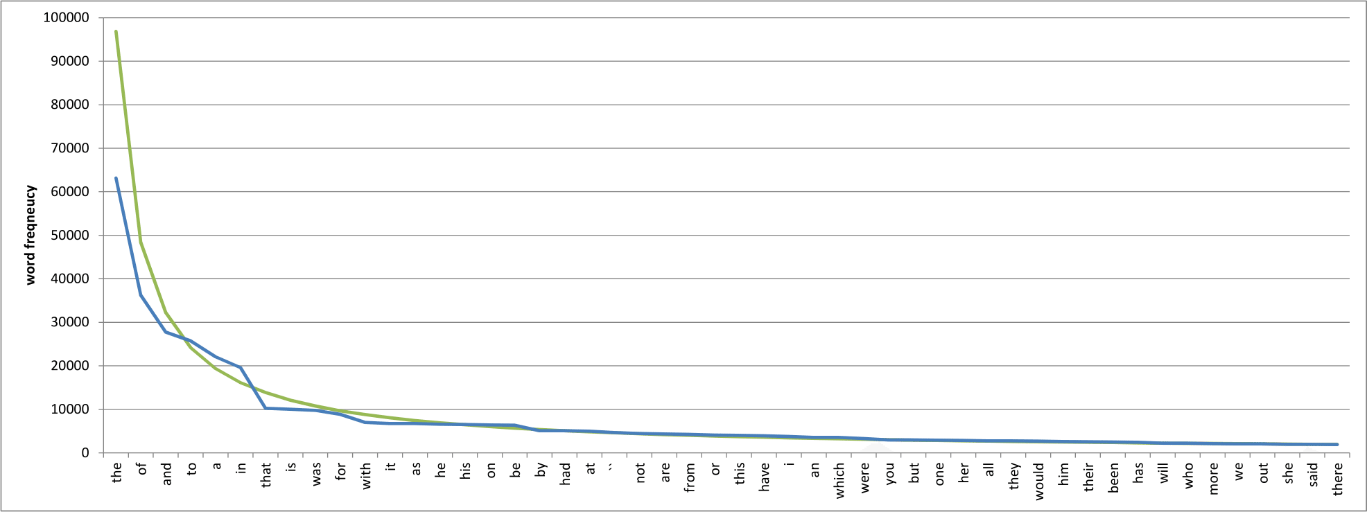
Before building the vocabulary, some preprocessing steps are common. One is to remove low-frequency words, a practice supported by Zipf’s law, which states that word frequency is inversely proportional to its rank. As shown in the following figure, if we keep all the unique tokens in the vocabulary, there will be many tokens with extremely low frequency, which will significantly inflate the vocabulary size and also potentially cause the overfitting issue (discussed in the last section of this lecture).
Another is to convert all text to lowercase to reduce the vocabulary size, though this can sometimes lead to ambiguity, for instance, between “Apple” the company and “apple” the fruit.
So far, there is no perfect tokenization method, in the sense of aligning with the semantic understanding of individual English words. Any choice of the tokenization method is essentially a tradeoff among many criteria, for example, the vocabulary size, the application domain, and the expressive power.
Section III: Case Study – Sentiment Analysis
Let’s consider a toy example for sentiment analysis with the following data:
| Example | Text (\( x \)) | Label (\( y \)) |
|---|---|---|
| Text 1 | I love coffee | Positive |
| Text 2 | I do not like tea | Negative |
| Text 3 | I like coffee | Positive |
A simple approach, known as the majority baseline, is to always predict the most frequent class. In this case, always predicting “Positive” would yield an accuracy of 66.7%.
A slightly more advanced rule-based classifier could count the number of positive and negative words in a text. For “I love coffee,” the presence of one positive word would lead to a “Positive” prediction. This is equivalent to a linear classifier with predefined weights for positive and negative words. For example, the weights could be set as follows:
| I | love | coffee | do | not | like | tea | |
|---|---|---|---|---|---|---|---|
| \( w_{\text{pos}} \) | 0 | 1 | 0 | 0 | 0 | 1 | 0 |
| \( w_{\text{neg}} \) | 0 | 0 | 0 | 0 | 1 | 0 | 0 |
The prediction is made by comparing the scores \( w_{\text{pos}}^{\top}x \) and \( w_{\text{neg}}^{\top}x \). For “I love coffee,” the bag-of-words vector is \( x = [1, 1, 1, 0, 0, 0, 0] \), resulting in \( w_{\text{pos}}^{\top}x=1 \), which is greater than \( w_{\text{neg}}^{\top}x=0 \).
However, many texts express sentiment without using obvious sentiment words. For example, in the following user review, we may agree this is a positive review even though the entire review has no positive sentiment words.
Its aroma was of earth and smoke. The first sip was an abrupt, bitter jolt that commanded my full attention. Any trace of morning fatigue vanished. I finished the entire cup without pause and immediately brewed another. This is the coffee I will be drinking from now on.
This highlights the need for learning-based classifiers that can automatically learn the importance of different words from data.
Section IV: Logistic Regression
A linear model for classification can be defined as:
\[h_y(x) = w_y^{\top}x + b_y\]Here, \( x \) is the bag-of-words vector, \( w_y \) represents the learnable classification weights for label \( y \), and \( b_y \) is the bias term for that label. A higher bias for a more frequent class can improve the model’s accuracy.
The linear decision function can be expressed in a probabilistic form as:
\[P(y\mid x) \propto \exp(w_y^{\top}x + b_y)\]To ensure that the probabilities for all labels sum to 1, the softmax function is used:
\[P(y\mid x) = \frac{\exp (w_y^{\top}x + b_y)}{\sum_{y'\in\mathcal{Y}}\exp(w_{y'}^{\top}x + b_{y'})}\]For binary classification tasks, the sigmoid function provides an alternative:
\(P(Y=\text{pos}\mid x) = \frac{1}{1 + \exp(-w^{\top}x)}\) In this case, the probability of the negative class is simply \( 1 - P(Y=\text{pos}\mid x) \).

The parameters of the model, \( W = {w_y; y\in\mathcal{Y}} \), are learned using Maximum Likelihood Estimation (MLE). The goal is to maximize the likelihood of observing the training data. For a training set of examples \( {(x^{(i)}, y^{(i)})}_{i=1}^{m} \), this is achieved by maximizing the log-likelihood function:
\[\max_{W} \sum_{i=1}^{m} \log P(y^{(i)}\mid x^{(i)}; W)\]In practice, this is often formulated as minimizing the negative log-likelihood (NLL). For more details, you can refer to section 3 of the demo code.
Section V: \( \ell_2 \) Regularization
\( \ell_2 \) regularization is a technique used to prevent overfitting. It adds a penalty term to the objective function, which discourages the model from learning excessively large weights. The modified objective function is:
\[\max_{W} \sum_{i=1}^{m} \log P(y^{(i)}\mid x^{(i)}; W) - \frac{1}{C}\sum_{y\in\mathcal{Y}}\|w_y\|_2^2\]In this equation, \( |w_y|_2 \) is the \( \ell_2 \) norm of the weight vector \( w_y \), and \( C \) is the regularization coefficient. A smaller value of \( C \) corresponds to stronger regularization.
A typical machine learning setup involves three datasets: a training set for learning the model parameters, a validation set for tuning hyper-parameters like \( C \), and a test set for the final evaluation of the model.
Overfitting occurs when a model performs well on the training set but poorly on the test set. For instance, with a large value of C (e.g., C=1000, indicating weak regularization), a model might achieve a training accuracy of 99.97% but a test accuracy of only 53.43%. This is because the model learns large weights for words that are not genuinely predictive of the class.
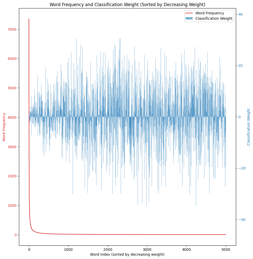
For example, the word “workings” might acquire a large positive weight from a single positive sentence, while “write” might get a large negative weight from one negative sentence. These learned weights do not generalize well to new data.
With stronger regularization (e.g., \( C = 0.01 \)), the model’s performance might be more balanced, such as a training accuracy of 62.57% and a test accuracy of 63.15%. Regularization helps to reduce overfitting by preventing the weights from becoming too large, which forces the model to rely on a broader range of features.
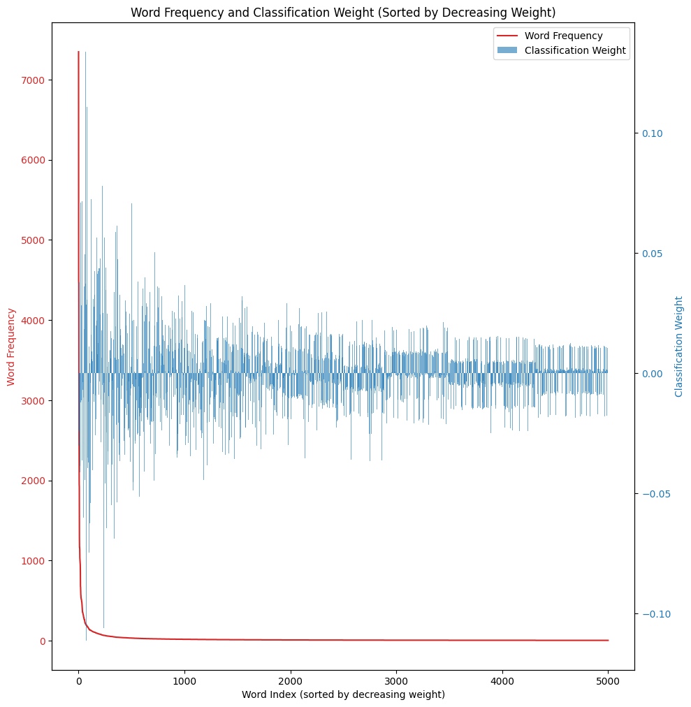
The table below compares the weights learned with and without regularization, illustrating how regularization leads to smaller and more reasonable weight values.
| interesting | pleasure | boring | zoe | write | workings | |
|---|---|---|---|---|---|---|
| Without Reg | 0.011 | -5.63 | 1.80 | -5.68 | -8.20 | 14.16 |
| With Reg | 0.16 | 0.36 | -0.21 | -0.057 | -0.066 | 0.04 |
In summary, regularization can reduce the correlation between class labels and noisy features, leading to a more robust and generalizable model.