Table of Contents
1. Review: Linear Functions
2. Perceptron
3. Logistic Regression
4. Linear Regression

---

1. Review: Linear Functions

In this lecture and some following lectures, we will talk about several linear predictors.

• Halfspace predictors (in section 2)
• Logistic regression classifiers (in section 3)
• Linear regression predictors (in section 4)
• Linear SVMs (in the lecture on support vector machines)
• Naive Bayes classifiers (in the lecture on generative models)

In the core of these linear predictors, it is a linear function

\[h_{w,b} = \langle w,x\rangle + b = \sum_{i=1}^{d}w_ix_i + b\]

where \(w\) is the linear weights, and \(b\) is the bias. If we rewrite \(w\) and \(x\) in the following forms

\[w\leftarrow (w_1,w_2,\dots,w_d,b)^{\top}; x \leftarrow (x_1,x_2,\dots,x_d,1)^{\top}\]

we can rewrite the linear function in a more compact form

\[h_{w}(x) = \langle w, x\rangle\]

Example (2-D Linear Function) Consider a two-dimensional case with \(w=(1,1,-0.5)\):

\[f(x) = w^{\top}x = x_1 + x_2 - 0.5\]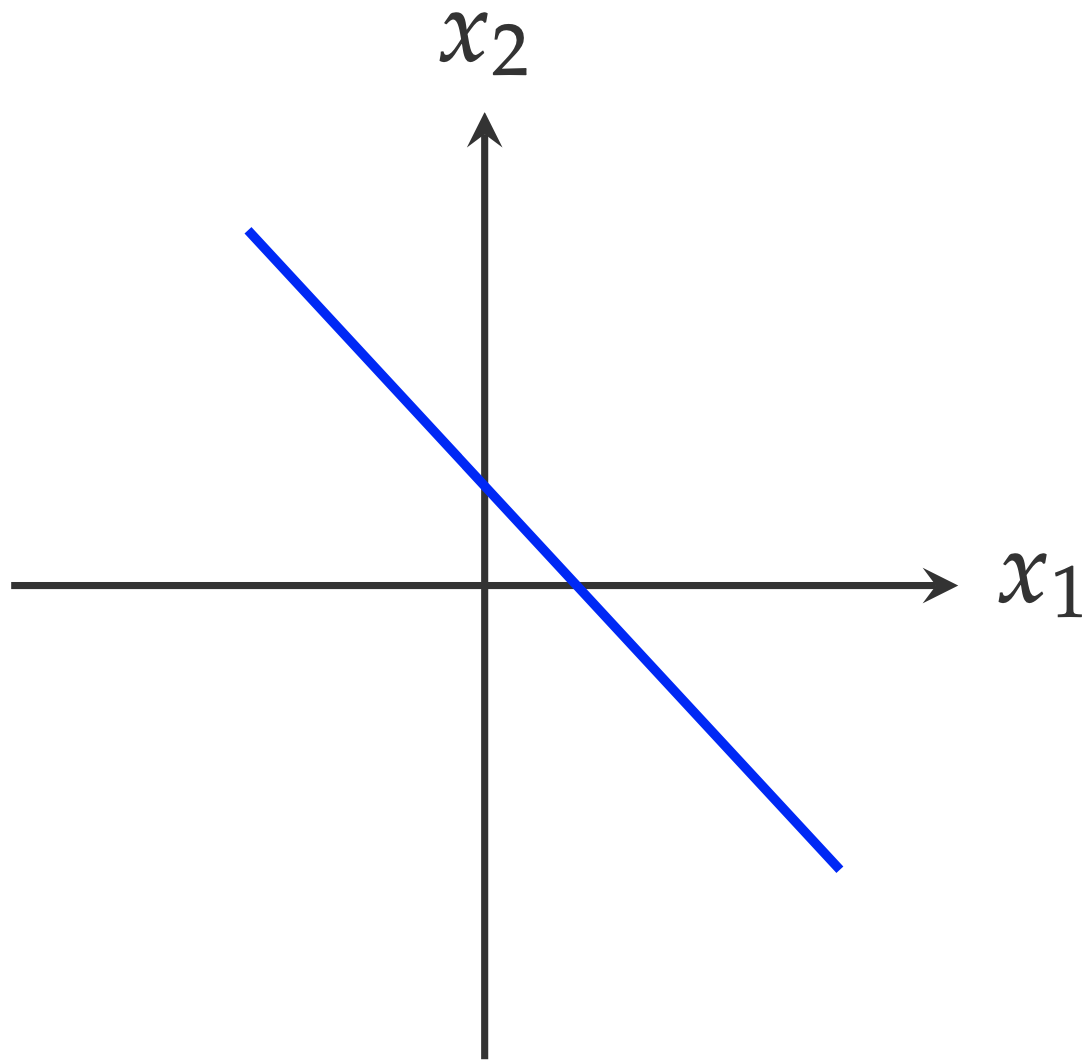

Different values of \(f(x)\) map to different areas on this 2-D space. For example, the following equation defines the blue line \(L\) in the figure:

\[f(x)=w^{\top}x = 0\]

For any two points \(x\) and \(x’\) lying on the line

\[f(x) - f(x') = w^{\top}x - w^{\top}x' = 0\]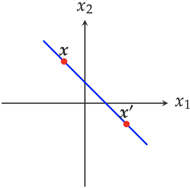

Furthermore,

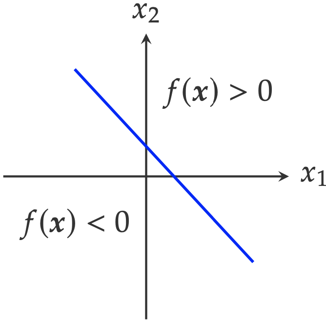
\[f(x) = x_1 + x_2 - 0.5 = 0\]

separates the 2-D space \(\mathbb{R}^2\) into two half-spaces.

From the perspective of linear projection, \(f(x)=0\) defines the vectors on this 2-D space, whose projections onto the direction $(1,1)$ have the same magnitude \(0.5\)

\[x_1 + x_2 - 0.5 = 0 \Rightarrow (x_1,x_2)\cdot\left(\begin{array}{c}1\\ 1\end{array}\right) = 0.5\]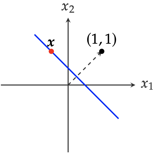

This idea can be generalized to compute the distance between a point and a line (e.g., in the case of computing the margin of a linear SVM classifier).

In generation, the distance of a point \(x\) to line \(L: f(x) = 0\) is given by

\[\frac{f(x)}{\|w\|_2} = \frac{\langle w,x\rangle}{\|x\|_2} = \langle\frac{w}{\|w\|_2},x\rangle.\]

---

2. Perceptron

For the domain set \(\mathcal{X}=\mathbb{R}^{d}\) and the label set \(\mathcal{Y}=\{-1,+1\}\), the halfspace hypothesis class is defined as

\[\mathcal{H}_{\text{half}} = \{\text{sign}(\langle w,x \rangle): w\in\mathbb{R}^{d}\}\]

which is an infinite hypothesis space. The sign function is defined as

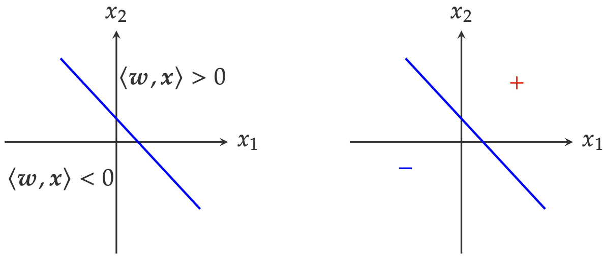
\[\text{sign}(x) = \left\{\begin{array}{ll} 1; x > 0\\ 0; x = 0\\ -1; x < 0\end{array}\right.\]

Based on the sign function, the hypothesis \(h\in\mathcal{H}_{\text{half}}\) with any given \(w\) will separate the input space \(\mathcal{X}\) into two halfspaces

\[h(x) = \left\{\begin{array}{ll} + 1; \langle w,x\rangle > 0\\ -1; \langle w,x \rangle < 0 \end{array}\right.\]

as shown in the following plots.

To demonstrate how to find a hypothesis \(h\) for a given classification case. Let’s first consider a simple 2-D classification problem.

Example (Linearly Separable Case) As shown in the following plot. The training set \(S\) consists of two classes (red and blue). The problem is finding a hypothesis \(h\) that can separate the examples in one class from the other. Intuitively, we can tell that there is definitely a hypothesis from \(\mathcal{H}_{\text{half}}\) that satisfies this requirement. In other words, the training set is linear separable.

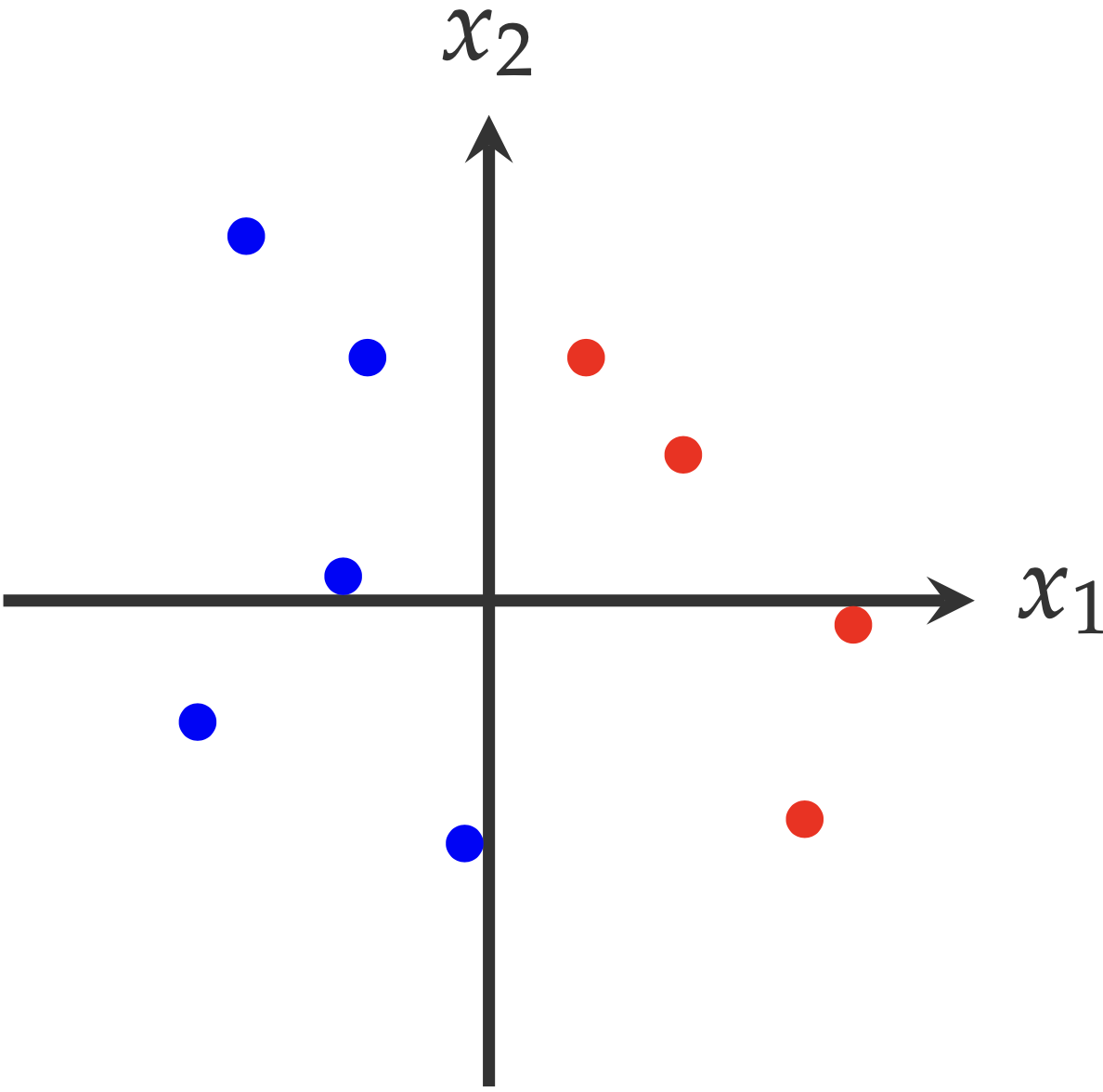
\(\Box\)

Note that the definition of linearly separable cases is defined with respect to the training set \(S\), not on the distribution \(\mathcal{D}\). Because based on the limited examples (in the training set \(S\)), we can never tell how the whole distribution \(\mathcal{D}\) looks like.

For a linearly separable case, there are several different algorithms that can learn (or identify) a hypothesis \(h\in\mathcal{H}_{\text{half}}\) that can well separate one class from the other. In this section, we will consider the simplest algorithm — the Perceptron algorithm, which is probably also the simplest algorithm in machine learning. Despite the simplicity, it contains the essential idea of learning algorithms.

Algorithm (Perceptron Algorithm) Here is a sketch of the Perceptron algorithm. The algorithm starts with zero weight \(w^{(0)}=(0,\dots,0)\) as shown in line 2. Then, in each iteration \(t\), the learning algorithm picks one example from the training set \(S\) (line 4). If the current classifier makes the wrong prediction on this example (line 5), the classification weight will be updated to push it to make the correct prediction next time.

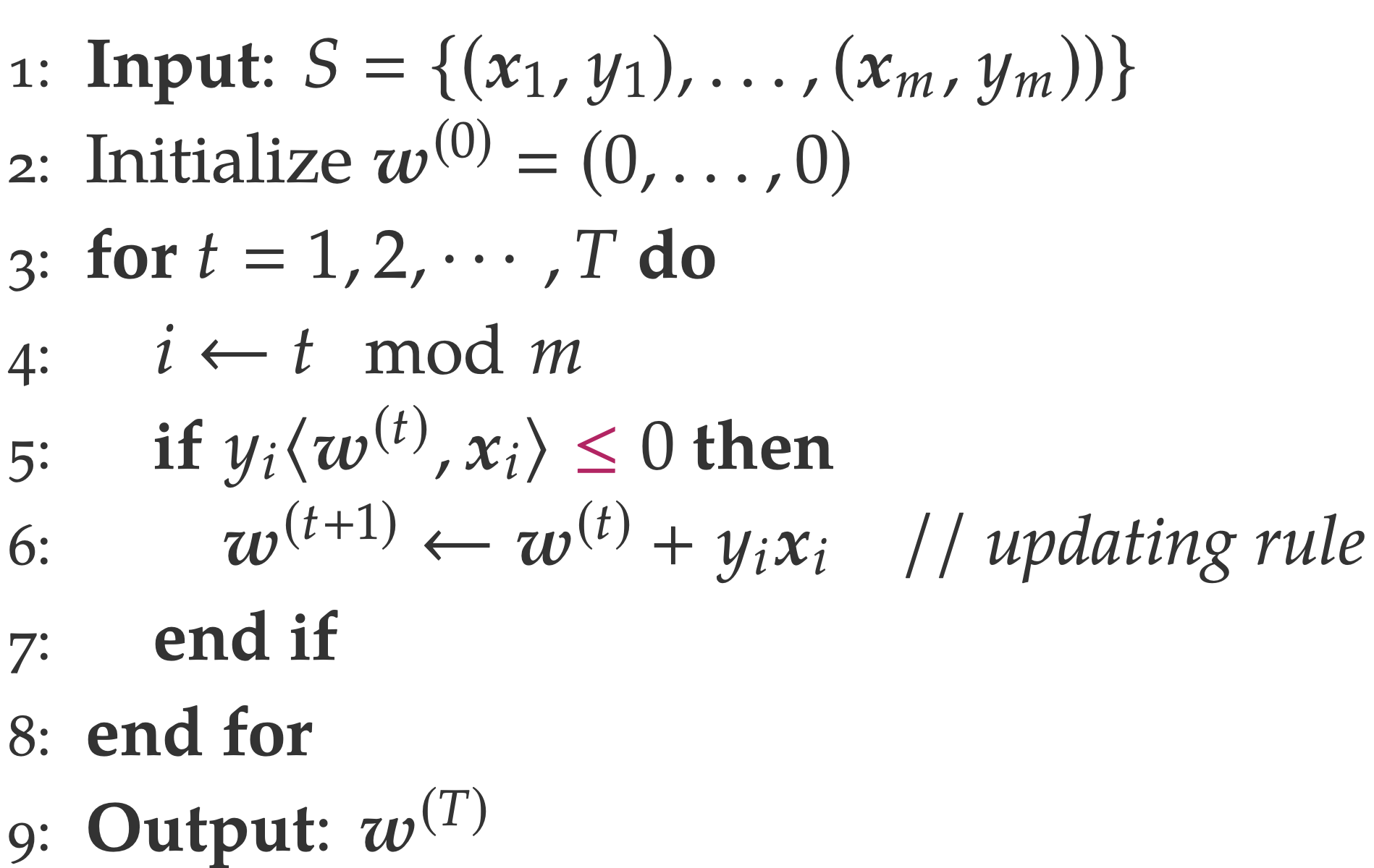
\(\Box\)

To better understand the updating rule

\[w^{(t+1)} \leftarrow w^{(t)} + y_ix_i\]

we need to answer two questions

1. How the updating rule can help?
2. How many updating steps does the algorithm need?

Answer to Q1: To answer the first question, let’s consider a specific case with \(y_i= +1\), for which the updating rule becomes

\[w^{(t+1)} \leftarrow w^{(t)} + x_i\]

To justify this updating rule, we can multiply \(x\) on both sides of the previous equation

\[\langle w^{(t+1)}, x_i\rangle = \langle w^{(t)}, x_i\rangle + \langle x_i,x_i\rangle = \langle w^{(t)}, x\rangle + \|x_i\|_2\]

Therefore, \(w^{(t+1)}\) gives a higher value on prediction \(x_i\) then \(w^{(t)}\), which push the classifier makes right prediction. Note that, the updating rule is also affected by the norm of \(x_i\), \(\|x_i\|^2\).

Answer to Q2: Regarding the second question, based on the answer to the first question and the fact that we know there always exists a hypothesis \(h\) from \(\mathcal{H}_{\text{half}}\) for linearly separable cases, intuitively the algorithm will stop in finite steps. Formally, this intuition is supported by the theorem of the Perceptron algorithm (Shalev-Shwartz and Ben-David, Theorem 9.1).

---

3. Logistic Regression

Similar to the previous section, we will start this section by introducing the hypothesis class of logistic regression. For binary classification, the hypothesis class is defined as

\[\mathcal{H}_{LR} = \{\sigma(\langle w,x\rangle): w\in\mathbb{R}^{d}\}\]

in which \(\sigma(\cdot)\) is the sigmoid function defined as \(\sigma(a) = \frac{1}{1+\exp(-a)}\). Assume \(\mathcal{Y}=\{-1,+1\}\), the decision rule of a logistic regression classifier is

\[y = \left\{\begin{array}{ll} + 1; h(x) > 0.5\\ -1; h(x) < 0.5\end{array}\right.\]

Although the definition of logistic regression has a non-linear function \(\sigma\), each \(h(x)\) is still a linear classifier. To verify this, let’s consider the decision boundary defined as \(h(x)\)

\[h(x) = 0.5\Rightarrow \exp(-\langle w,x\rangle) = 1\Rightarrow \langle w,x\rangle = 0\]

Therefore, the decision boundary is a linear function of \(x\). In other words, \(h(x)\) is a linear classifier.

To align with the half-space hypothesis class, we can re-define a hypothesis in \(\mathcal{H}_{LR}\) by explicitly introducing the label \(y\) into the definition.

\[h(x,y) = \frac{1}{1+\exp (-y\langle w,x\rangle)}\]

and the corresponding decision rule becomes

\[y = \left\{\begin{array}{ll} + 1; h(x,+1) > h(x,-1)\\ -1; h(x,+1) < h(x,-1)\end{array}\right.\]

This is mostly for mathematical convenience, and it won’t change any conclusion we have about logistic regression. For example, each hypothesis is still a linear classifier.

The loss function of \(\mathcal{H}_{LR}\) is defined as

\[L(h,\{(x,y)\}) = -\log\frac{1}{1+\exp(-y\langle w,x\rangle)} = \log(1 + \exp(-y\langle w,x\rangle))\]

Intuitively, minimizing the loss function \(L\) will increase the value of $h$ on the training example \((x,y)\). However, unlike the 0-1 loss used by the \(\mathcal{H}_{\text{half}}\), the definition of the loss function for \(\mathcal{H}_{LR}\) is not straightforward, at least from the perspective of classification. The statistical motivation of this loss function will be explained in the second part of this section.

Moving forward with this definition, the empirical risk of learning a logistic regression model is defined as

\[L(h, S) = \frac{1}{m}\sum_{i=1}^{m}\log (1+\exp(-y_i\langle w,x_i\rangle))\]

where \(S=\{(x_1,y_1)\dots, (x_m,y_m)\}\) is the training set. To learn a hypothesis \(h\) is equivalent to finding a \(w\) that can minimize the empirical loss

\[\hat{w} \leftarrow \text{argmin}_{w'} L(h_{w'}, S)\]

With \(L(h,S)\) as a differentiable function, the optimization problem can be solved by gradient-based optimization methods.¹

Specifically, the gradient of \(L(h_w,S)\) with respect to \(w\)

\[\frac{d L(h_w,S)}{dw} = \frac{1}{m}\sum_{i=1}^{m}\frac{\exp (-y_i\langle w,x_i\rangle)}{1 + \exp(-y\langle w,x_i\rangle)}\cdot (-y_ix_i)\]

To minimize the loss, the gradient-based updating rule is

\[w^{\text{new}} = w^{\text{old}} - \eta\cdot \frac{d L(h_w,S)}{dw} = w^{\text{old}} + \frac{\eta}{m} \frac{\exp (-y_i\langle w,x_i\rangle)}{1 + \exp(-y\langle w,x_i\rangle)}\cdot (-y_ix_i)\]

where \(\eta\) is called learning rate, which controls the updating step size. To understand why this algorithm works, we need to understand two components in the above updating equation: for each training example \((x_i,y_i)\)

• the component \((y_ix_i)\) is the exactly the same as the Perceptron algorithm as discussed in the previous section. That means, the updating rule is following the same motivation of updating the classification weight \(w\)
• the component \(\frac{\exp (-y_i\langle w,x_i\rangle)}{1 + \exp(-y\langle w,x_i\rangle)}\) shows the difference between this updating rule and the Perceptron updating rule. To be specific, the magnitude of updating is proportional to the prediction value (probability) of the opposite label. Intuitively, if the prediction probability on the opposite label is higher, then the updating on the classification weight will also be more aggressive — to make sure the model can make a better decision next round.

Besides, the hypothesis class also provides us a good opportunity to explain statistical machine learning. What we need to is just re-define a few things using the terminology from Statistics.

Model formulation: from a probabilistic view, a hypothesis in \(\mathcal{H}_{LR}\) defines the probability of a possible label \(y\) given the input \(x\)

\[p_w(Y=y\mid x) = h_w(x,y) = \frac{1}{1 + \exp (-y\langle w,x\rangle)}\]

where \(Y\) is a random variable with possible values \(Y\in{-1, +1}\). Then the previous decision rule can be re-formulated as

\[y=\left\{ \begin{array}{ll} + 1; \text{if}~p(Y=+1\mid x) > p(Y=-1\mid x)\\ -1; \text{if}~p(Y=+1\mid x) < p(Y=-1\mid x)\end{array}\right.\]

Model learning: Given the training set \(S=\{(x_1,y_1), \dots, (x_m, y_m)\}\), the likelihood function of \(w\) is defined as

\[\text{Lik}(x) = \prod_{i=1}^{m} p_w(y_i\mid x_i).\]

Equivalently, the log-likelihood function is defined as

\[\ell(w) = \sum_{i=1}^{m}\log p_w(y_i\mid x_i)=-\sum_{i=1}^{m}\log (1 + \exp(-y\langle w, x_i\rangle))\]

From perspective of statistical machine learning, one way of learning \(w\) is to maximize the (log-)likelihood function

\[\text{argmax}_{w}\ell(w)=\text{argmax}_{w}-\ell(w)=\text{argmax}_{w} L(h_w,S)\]

Therefore, it is equivalent to minimize the loss function \(L(h_w, S)\) defined before.

---

4. Linear Regression

---