Table of Contents
1. Key Concepts
2. Data Generation Process
3. True Risk and Empirical Risk
4. Empirical Risk Minimization
5. Finite Hypothesis Classes
6. PAC Learning
7. Agnostic PAC Learning

---

1. Key Concepts

Let’s consider a simple machine learning problem. The following figure shows the examples collected from two classes: positive (+) and negative (-). A machine learning question that we would like to answer is: Given the examples as illustrated in the following figure, what is the shape/size of the area where the positive example (+) comes from?

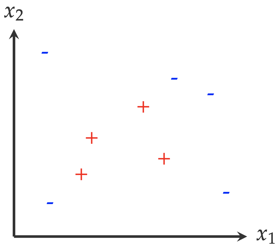
To answer this question, we have to make certain assumptions. For example, we have to assume these data points are representative enough¹: all positive examples are surrounded by negative examples, and there are no positive examples beyond the region where negative examples are distributed. Honestly, there is no evidence to support this assumption. However, without this assumption, we cannot even get started to think about an answer.

With that assumption, we can move forward to answer the question in two steps:

1. Which shape is the underlying distribution of positive examples? Here are some candidate answers
   • Triangle, with positive label inside
   • Rectangle, with positive label inside
   • Circle, with positive label inside
   • A shape that I cannot describe, with positive label inside
2. What is the size of that shape?

In future lectures, we are going to mention the keyword assumption many times. This is a key to understanding machine learning (and statistical modeling). In other words, using machine learning to solve problems, we have to start from certain assumptions to move forward, either explicitly or implicitly.

This simple example gives us enough information to characterize a machine learning problem. In the following lectures, we will use the following terminology to describe any machine learning problem.

• Domain set (or, Input space) \(\mathcal{X}\): the set of all possible examples
  • In the toy example, without further constraint, \(\mathcal{X}\) can be the whole 2-D plane \(\mathcal{X}=\mathbb{R}^2\);
  • Each point \(x\) in \(\mathcal{X}\), \(x\in\mathcal{X}\), is called an instance or example.
• Label set (or, Output space) \(\mathcal{Y}\): the set of all possible labels
  • In the toy example, \(\mathcal{Y}\in\{+,-\}\);
  • In the following lectures, without further clarification, we will assume a label set always contains two elements. In addition to the previously defined \(\mathcal{Y}\), it can also take one of the following forms: \(\{0,1\}\) or \(\{+1,-1\}\).
• Training set \(\mathcal{S}\): a finite sequence of pairs in \(\mathcal{X}\times\mathcal{Y}\), represented as \(\{(x_1,y_1),(x_2,y_2),\dots,(x_m,y_m)\}\) with \(m\) as the size of the training set. Sometimes, we will use \(\{(x_i,y_i)\}_{i=1}^{m}\) for short.
  • In the toy example, the training set includes all the examples observed in that figure;
  • In machine learning, training set is always the starting point, as the problem often has an infinite domain set, like the one demonstrated by the toy example.
• Hypothesis class (or, Hypothesis space) \(\mathcal{H}\): a set of functions that map instances to their labels
  • Each element \(h\) in the hypothesis space \(\mathcal{H}\), \(h\in\mathcal{H}\) is called a hypothesis;
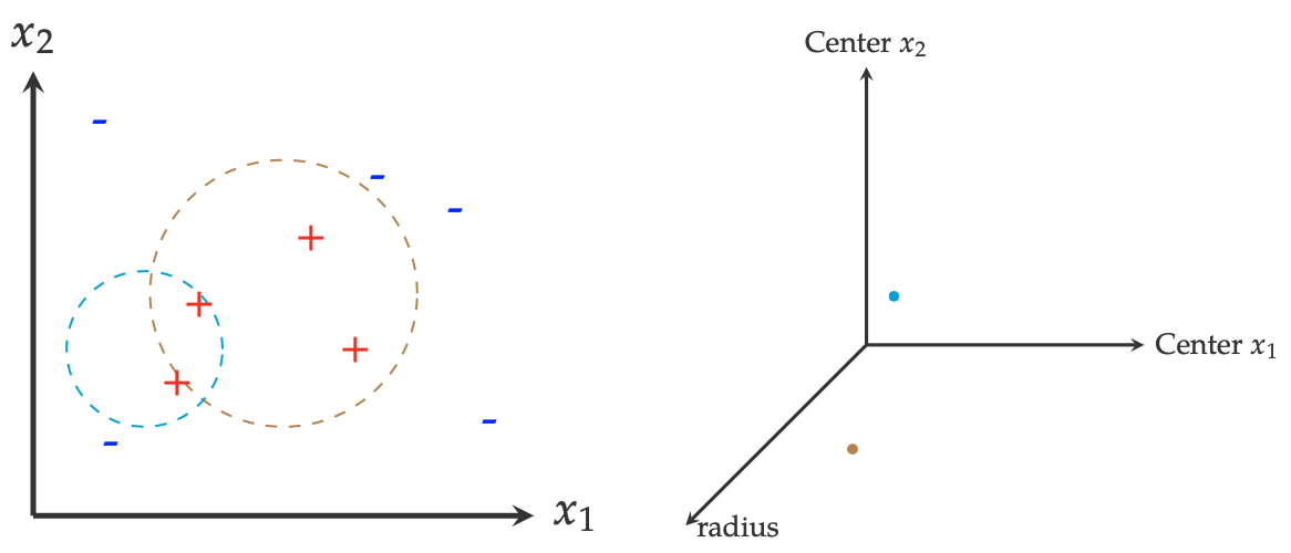
  • In the toy example, by answering the first question, we equivalently pick a hypothesis class. For example, \(\mathcal{H}_{\text{circle}}=\{\text{all the circles, with positive label inside}\}\);
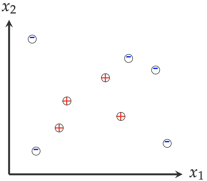
  • There are two different ways to describe a hypothesis class (and its hypotheses). As shown in the following figure, one is from the input space \(\mathcal{X}\) and the other is in the hypothesis space. The left figure two hypotheses in the original input space. In the hypothesis space \( \mathcal{H}_{\text{circle}} \), any hypothesis \( h \) can be described by its coordinates \((x_1,x_2)\) and its radius \(r\), as shown in the right figure. In other words, in the hypothesis space, each hypothesis \(h\) is represented as a dot.
    
• A (machine) learner: an algorithm \(A\) that can find an optimal hypothesis from \(\mathcal{H}\) based on the training set \(S\)
  • In this lecture note, the optimal hypothesis is represented as \(A(S)\). How to measure its optimality is a central topic in machine learning;
  • Not every hypothesis space has a corresponding algorithm \(A\). If \(A\) exists, then the corresponding hypothesis space is learnable.

---

2. Data Generation Process

In this section, we will give a formal discussion on some phenomena in machine learning. The starting point of this discussion is to connect the first three concepts discussed in the previous section:

• Domain set \(\mathcal{X}\),
• Label set \(\mathcal{Y}\),
• Training set \(S\).

In machine learning, these three concepts can be naturally connected with a hypothetical process, called data generation process. In general, a typical data generation process to describe \(\mathcal{X}\), \(\mathcal{Y}\), and \(S\) is

1. define a probability distribution \(\mathcal{D}\) over the domain set \(\mathcal{X}\);
2. sample an instance \(x\in\mathcal{X}\) according to \(\mathcal{D}\);
3. annotate it using the labeling function (aka, the oracle) \( f \) as \( y=f(x) \).

Repeat the last two steps until we have the whole training set \( S=\{ (x_i,y_i) \}_{i=1}^{m} \).

Although this is by no means the actual data generation process where we collect data in machine learning practice, this over-simplified hypothetical process provides us a way to both clarify some concepts and design further examples for discussion. Later, with the probabilistic language, it can also be used a powerful probabilistic modeling strategy, called generative modeling.

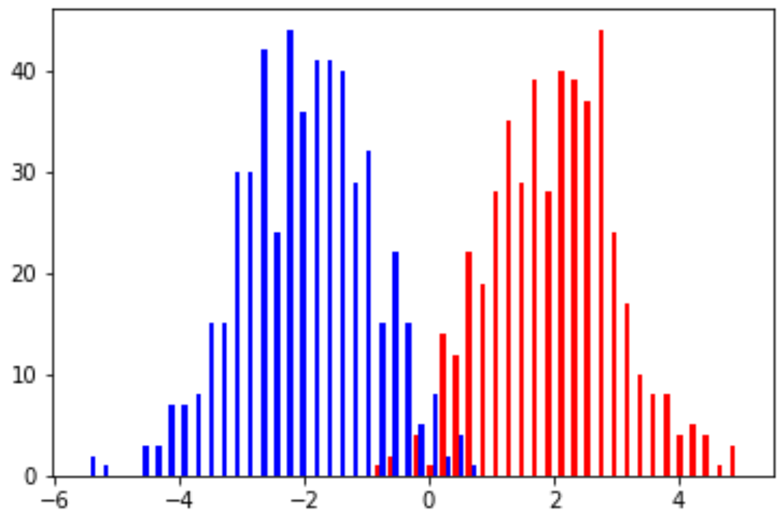
Example (Mixture of Gaussians): Assume the data distribution \( \mathcal{D} \) over the domain set \( \mathcal{X} \) is defined as

\[p(x) = \frac{1}{2}\mathcal{N}(x;2,1) + \frac{1}{2}\mathcal{N}(x; -2, 1)\]

where \( \mathcal{N}(x;\mu,\sigma^2) \) is a Gaussian distribution with mean \( \mu \) and variance \( \sigma^2 \). Therefore, \( p(x) \) is a mixture of two components of Gaussian distribution and also a legitimate probability density function, as \( \int_x p(x) dx = 1 \). With this probability distribution, one example of the last two steps can be

• randomly select a component, and sample \( x \) from it;
• label \( x \) based on which component it comes from. In other words, the labeling function is defined as

\[f(x) = \left\{\begin{array}{ll}\text{positive}; & x~\text{from the first component}\\ \text{negative}; & x~\text{from the second component}\end{array}\right.\]

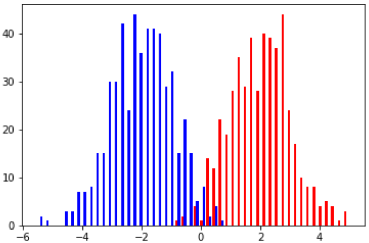
The following figure shows the histogram of sampled examples, with examples in each class following a Gaussian distribution. Note that, with the defined mean and variance values, it is unavoidable to have overlapped areas between these two classes.

\( \Box \)

In the following sections, we will continue our discussion from the aspect of learning, which involves the last two concepts that we discussed in the previous section

• Hypothesis class \( \mathcal{H} \)
• A machine learner \( A \)

Recall the definition of a machine learner:

“an algorithm \( A \) that can find an optimal hypothesis from \( \mathcal{H} \) based on the training set \( S \)”

To continue our discussion, we need to explain what is an optimal hypothesis? In other words, what are the criteria of optimality when finding a hypothesis from a given class \(\mathcal{H}\)?

---

3. True Risk and Empirical Risk

For a given hypothesis \(h\), a classification error on \(x\) is defined as the mismatch between the prediction from hypothesis \(h\) and from the labeling function \(f\),

\[h(x)\not= f(x)\]

In general, the error of a classifier is defined as the probability of classification error on a randomly generated example \(x\in\mathcal{X}\)

\[L_{\mathcal{D},f}(h) = P_{x\sim\mathcal{D}}[h(x)\not= f(x)]\]

The intuitive explanation of the right-hand side of this definition is that, for a randomly sampled \(x\) from the distribution \(\mathcal{D}\), the probability that \(h(x)\) and \(f(x)\) do not match.

Note that, the error of a classifier \(L_{\mathcal{D},f}(h)\) is measured with respect to the “true” data distribution \(\mathcal{D}\) and the “true” labeling function \(f\). Therefore, it is also called true error (or true risk). From a machine learning perspective, it measures how the hypothesis \(h\), selected from limited training example \(S\), performs on the whole domain set \(\mathcal{X}\). Therefore, this error sometimes is also called the generalization error.

Example (Mixture of Gaussians, Cont.): Continue the previous example with two components of Gaussian distributions. Also, assume we have the same labeling function \(f\). The data distribution can be shown in the following figure, with red indicating positive label and blue indicating negative label.

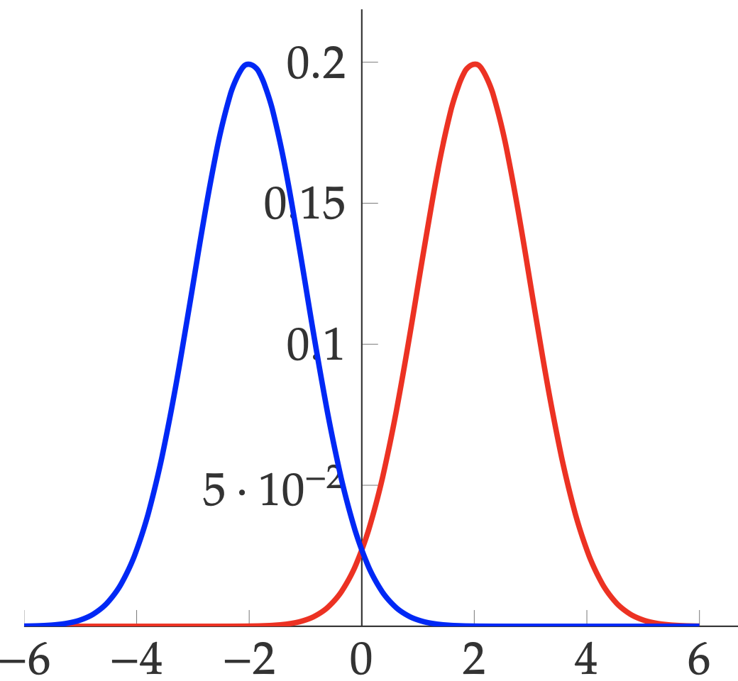
If hypothesis \(h\) is defined as

\[h(x) = \left\{\begin{array}{ll} +1 & p(+1\mid x) \geq p(-1 \mid x)\\ -1 & \text{otherwise}\end{array}\right.\]

Then, what is the true error \(L_{\mathcal{D},f}(h)\) is the area under the red curve when \(x < 0\) and the area under the blue curve when \(x > 0\). In other words, it is the probability of a positive example falls into the region of \(x < 0\) and the probability of a negative example falls into the region of \(x > 0\).

\(\Box\)

Note that the definition of true risk indicates it is not operational. Recall that, the definition \(L_{\mathcal{D}, f}(h)\) relies two factors: (i) the true data distribution \(\mathcal{D}\) and (ii) the labeling function \(f\). However, both of them are unknown. As in machine learning, the only thing we know is the training set \(S\). Therefore, we need the empirical risk \(L_{S}(h)\) as an approximation to the true risk \(L_{\mathcal{D}, f}(h)\).

The definition of the empirical risk (or empirical error, training error) is defined as

\[L_S(h) = \frac{|\{i\in[m]: h(x_i)\not y_i\}|}{m}\]

where \([m] = \{1,2,\dots,m\}\) and ((m\) is the total number of training examples. The numerator \( |{ i\in[m]: h(x_i)\not=y_i}| \) is the number of examples that the predictions do not match the true label \(y_i\).

Example (Mixture of Gaussians, Cont.): For the hypothesis \(h\) defined in the previous example, the empirical error is the ratio between

• the total number of (1) positive examples in the region \(x < 0\) and (2) negative examples in the region \(x > 0\), and
• the total number of examples (\(m = 1000\) in this case)

\(\Box\)

After clarifying the criterion of optimality (true risk) and its proxy (empirical risk), in the next section, we will move the learning paradigm – empirical risk minimization.

---

4. Empirical Risk Minimization

Given the training set \(S\) and a hypothesis class \(\mathcal{H}\), the empirical risk minimization of finding an optimal hypothesis \(h\) is defined as

\[h\in\text{argmin}_{h'\in\mathcal{H}}L_S(h')\]

where the empirical risk \( L_S(h) \) is defined in the last section. Note that \(\text{argmin}_{h'}L_S(h')\) represents a set of hypotheses that can minimize the empirical risk. One example is a linear separable case discussed in the next lecture, which often has an infinite number of hypotheses that can satisfy \(L_{S}(h)=0\).

As shown in the following example, if we can make a hypothesis space large enough, there is always at least one hypothesis that can make \(L_S(h)\) close to zero.

Example: Consider that 2-D classification problem at the beginning of this lecture, with an unconstrained hypothesis space \(\mathcal{H}\), there is always a hypothesis as defined in the following that can minimize the empirical risk to be \(0\)

\[h_S(x) = \left\{ \begin{array}{ll} y; & \text{if}~(x = x_i)\wedge (x_i\in S)\\ 0; & otherwise \end{array} \right.\]

As illustrated in the following figure, for any given \(x_i\in S\), \(h_S(x)\) will precisely predict the label of \(x_i\) as \(y_i\), no matter how many examples in \(S\). However, although \(L_S(h_S) = 0\), the hypothesis \(h_S\) defined in the above equation does not have any prediction power on any new example.

\(\Box\)

This example is just an illustration of one typical learning phenomenon, called overfitting. In machine learning, when a hypothesis gives (nearly) excellent performance on the training set but poor performance on the whole distribution \(\mathcal{D}\), we call this hypothesis overfits the training set. Recall the difference between empirical risk \(L_{\mathcal{D}, f}(h)\) and true risk \(L_S(h)\), overfitting means hypothesis \(h\) yields a big gap between \(L_{\mathcal{D}, f}(h)\) and \(L_S(h)\).

As implied in the above example, one way to eliminate overfitting is to somehow constrain the size of a hypothesis class. In the next lecture, we will start from the most straightforward strategy of constraining the size of a hypothesis class — considering a hypothesis class with finite hypotheses.

In a future lecture, once we have another way of measuring the capacity of hypothesis classes, we will introduce other strategies to solve the problem of overfitting.

---

5. Finite Hypothesis Classes

To give a specific example of learning with finite hypothesis class, let us consider the following simple learning problem:

• Domain set \( \mathcal{X}=[0,1]\)
• Distribution \( \mathcal{D} \): the uniform distribution over \( \mathcal{X} \)
• Label set \( \mathcal{Y}={-1,+1} \)
• Labeling function \( f \)

\[f(x) = \left\{\begin{array}{ll}-1; 0\leq x < b\\ + 1; b \leq x\leq 1\end{array}\right.\]

with \( b=0.2 \) in the following discussion. The learning problem discussed in this section is that, given a set of training examples \( S=\{(x_1,y_1),\dots (x_m,y_m)\} \), find the value of \( b \).

To be specific, can we find the value of \( b \) based on a training set?

To answer this question from the perspective of machine learning, we have to pretend that we don’t know the ground-truth value of \( b \). In other words, our guess of \( b \) will only be based on the training set. The answer to the question mentioned above relies on two factors:

1. the selection of a hypothesis class
2. the representativeness of a training set

As we will see in the following example, even for a simple learning problem, learning the value \( b \) requires a perfect match between these two factors.

Example (1-D Classification) To make the learning problem simpler, let’s consider a hypothesis class with finite hypotheses. Specifically, the hypothesis class is defined as

\[\mathcal{H}_{\text{finite}} = \{ h_i : i\in\{1,\dots,9\}\}\]

with each \( h_i \) is defined as

\[f(x) = \left\{\begin{array}{ll}-1; 0\leq x < \frac{i}{10}\\ + 1; \frac{i}{10} \leq x\leq 1\end{array}\right.\]

It is not difficult to see that the size of this hypothesis class is \( |\mathcal{H}_{\text{finite}}| = 9 \).

\( \Box \)

Given a finite hypothesis class, a natural question is whether the hypothesis is big enough to include the hypothesis that we need to find? To answer this question, we need the following assumption.²

Realizability Assumption: there exists \(h^{\ast}\in\mathcal{H}_{\text{finite}}\) such that \(L_{\mathcal{D}, f}(h^{\ast}) = 0\).

\(\Box\)

When we consider this assumption holds, it means we think there is a hypothesis in \(\mathcal{H}_{\text{finite}}\) that can minimize the true error \(L_{\mathcal{D},f}\) to 0. Since we have the prior knowledge of \(b\), we can tell that \(\mathcal{H}_{\text{finite}}\) statisfies the realizability assumption.

In addition, this assumption is only about the existence of such a hypothesis. Whether we can find the hypothesis \( h^{\ast} \) will rely on the specific learning algorithm \( A \). In the case of finite hypothesis space, a simple enumeration algorithm will certainly do the job. Although we introduce this assumption in the context of finite hypothesis classes, this assumption is also useful when analyzing infinite hypothesis classes.

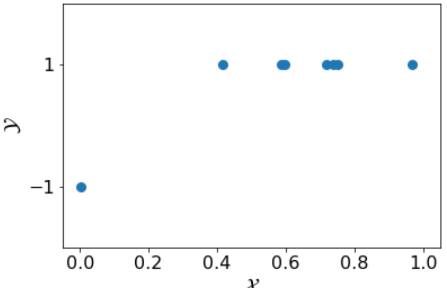
Example (1-D Classification, Cont.) Given the following training set with only eight examples, the simple algorithm \( A \) of enumerating all candidate hypotheses will identify the optimal hypothesis \( h^{\ast} = 0.2 \). Other learning algorithms with more time efficiency also exist, such as binary search. Whichever algorithm that we are going to use, with the training set \( S \) and the finite hypothesis class \( \mathcal{H}_{\text{finite}} \), it will identify the hypothesis \( h_2 \). This is exactly the labeling function \( f \).

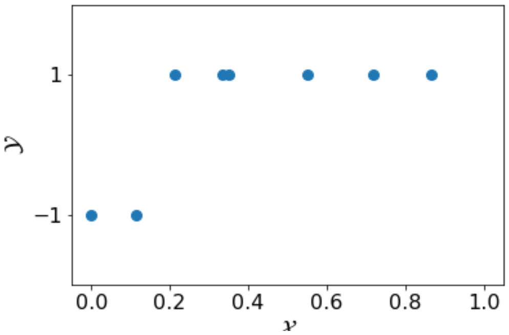
Now, let consider the following training set \( S’ \). With the same size as \( S \), \( S’ \) does not have any negative examples, which makes learning the value of \( b \) impossible.

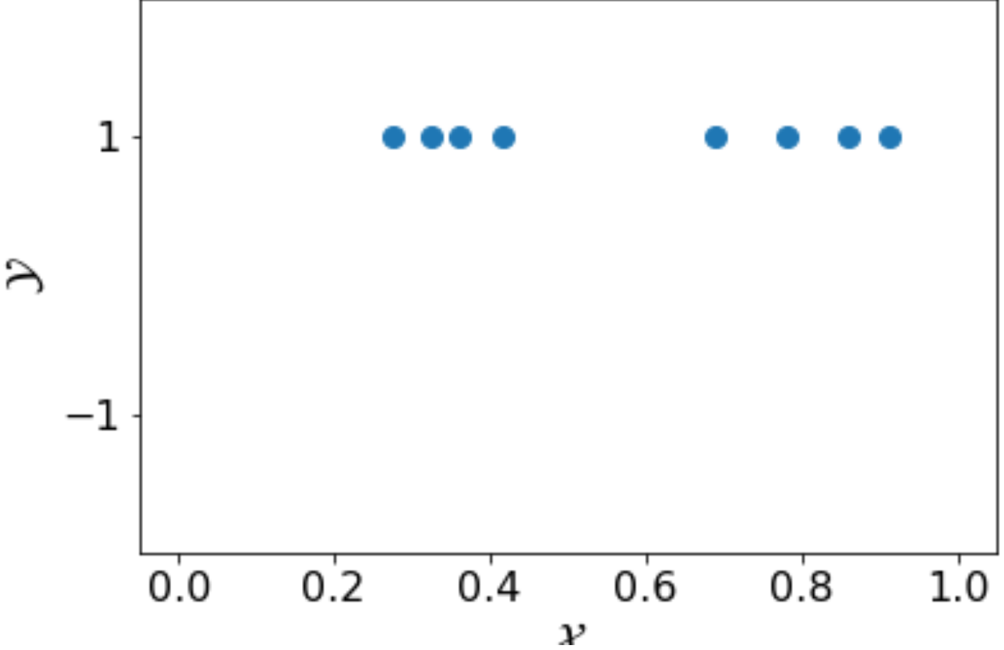
Example training sets like \( S’ \) are called non-representative examples. In machine learning, to take the possibility of having a non-representative training set into consideration, we need to relax our constraint of learning and let the learning algorithm fail with a small probability \( \delta \).

Furthermore, consider the following training set \( S’’ \), which again has the same number of training examples as in \( S \).

With \( S’’ \), both \( h_1 \) and \( h_2 \) will minimize the empirical error to 0. In other words, the learning algorithm cannot distinguish \( h_1 \) from \( h_2 \). If the algorithm happens to choose \( h_1 \) and stop the training, then we will have \( L_{S’’}(h_1) =0 \) but \( L_{\mathcal{D},f}(h_1) \not= 0 \). To deal with the situation like this, we need further relax our constraint and let \( L_{\mathcal{D}, f} \leq \epsilon\).

\( \Box \)

In this section, we use the example of learning with finite hypothesis class to demonstrate different situations that the learning algorithm may run into. As there is no guarantee that a learning algorithm can always find the ground-truth labeling function (even in a simple learning problem, as we demonstrated above), we need to relax the constraints and let the algorithm fail with a small probability (\( \delta \)) or find an imperfect hypothesis (with the true error less than \( \epsilon\)).

In the next section, we will use these two parameters to formally define learnability.

---

6. PAC Learning

We will keep the realization assumption in the discussion of this section and remove it in the next section. Although it is a strong assumption, with it, we don’t need to worry about whether a hypothesis class is in the right size for the time being — at least it has a hypothesis \( h^{\ast} \) that can minimize the true error to 0.

In this section, we will introduce the concept of learnability: what is learnable and when we call it is learnable. Specifically, we will introduce this concept with the framework of probably approximately correct (PAC) learning.

Before we give the rigorous definition, let’s introduce a simplified version first:

Definition (PAC Learnability, Simplified) A hypothesis class \(\mathcal{H}\) is PAC learnable, if there exists a learning algorithm \(A\) with the following property:

• for every distribution \(\mathcal{D}\) over \(\mathcal{X}\), and
• for every labeling function \(f: \mathcal{X}\rightarrow {0,1}\)

with enough training examples, the algorithm returns a hypothesis \(h\) such that with a large probability, \(L_{\mathcal{D},f}(h)\) is arbitrarily small.

\(\Box\)

Here are some important pieces of information in this definition

• the learnability is defined on the hypothesis class, not the learning task. Taking sentiment classification with Amazon reviews as an example, learnability is not about whether we can solve this classification task, rather about learning a classifier from a pre-defined class for this task.
• for a given domain set \(\mathcal{X}\), the learnability is defined on every distribution and every labeling function
• the assumption “with enough training examples” is about the sample complexity issue in machine learning. Recall the example of 1-D classification discussed in the previous section, and we don’t know whether eight examples in that case are sufficient or not. Machine learning theory will address this issue with some estimates on sample complexity
• the phrases “large probability” and “arbitrarily small” mean PAC learning does not require always finding the perfect hypothesis. As long as there is a large probability of finding a \(h\) close enough to the labeling function, it is fine.

With these explanations, now we can introduce the formal definition of PAC learning, which is nothing but describing the previous definition in a mathematical form:

Definition (PAC Learnability): A hypothesis class $\mathcal{H}$ is PAC learnable, if there exists a function \(m_{\mathcal{H}}: (0,1)^2\rightarrow\mathbb{N}\) and a learning algorithm with the following property:

• for every distribution \(\mathcal{D}\) over \(\mathcal{X}\)
• for every labeling function \(f:\mathcal{X}\rightarrow {0,1}\)
• for every \(\epsilon, \delta\in (0,1)\)

if the realizability assumption holds with respect to \(\mathcal{H}, \mathcal{D}, f\), then when running the learning algorithm on \(m\geq m_{\mathcal{H}}(\epsilon, \delta)\) i.i.d. examples generated by \(\mathcal{D}\) and labeled by \(f\), the algorithm returns a hypothesis \(h\) such that

\[P(L_{\mathcal{D},f}\leq \epsilon) > 1 - \delta.\]

\(\Box\)

The major difference between this full version and the previous simplified version

• instead of saying “large probability” and “arbitrarily small”, the full definition explicitly use \(\epsilon\) and \(\delta\) to describe the meaning
• instead of saying “enough training examples”, the full definition formally introduce the sample complexity lower bound \(m_{\mathcal{H}}(\epsilon,\delta)\), which is a function of \(\epsilon\) and \(\delta\). Intuitively, with smaller \(\epsilon\) and \(\delta\), we need a large \(m_{\mathcal{H}}\). Estimating sample complexity lower bound is an important task in machine learning theory.

For finite hypothesis classes, we can calculate the sample complexity lower bound as (for the derivation of this lower bound, please refer to (Shalev-Shwartz and Ben-David, 2014; Corollary 2.3)

\[m_{\mathcal{H}} = \frac{\log(|\mathcal{H}|/\delta)}{\epsilon}\]

Given the size of a hypothesis class and specific values of \(\epsilon\) and \(\delta\), we can calculate the sample complexity lower bound as demonstrated in the following example

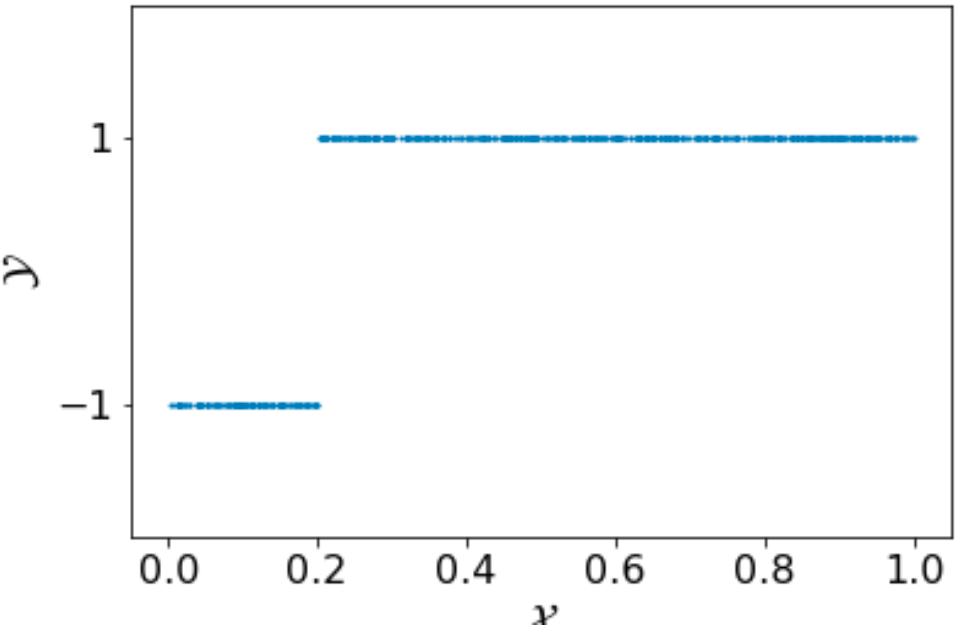
Example (Sample Complexity of 1-D Classification) With the following choices of \(\mathcal{H}\), \(\epsilon\) and \(\delta\):

• The size of the hypothesis class \(\mathcal{H}\): 100
• Confidence parameter: \(\delta=0.1\)
• Accuracy paramter: \(\epsilon=0.01\)

we have \(m_{\mathcal{H}} \approx 691\). And here is one training set with 691 examples sampled with the labeling function (\(b=0.2\)). Without running a learning algorithm, it is clear that we can identify the boundary value very close to \(b\).

\(\Box\)

Of course, the discussion so far is under the assumption of realizability. In the next section, we will consider the PAC learning without this assumption.

---

7. Agnostic PAC Learning

As we discussed before, the Realizability Assumption is unrealistic in many applications. For example, in image classification

• we don’t even know whether there exists a labeling function \(f\). As a matter of fact, even human annators may not agree with each other on certain images;
• even there exists a labeling function, we still don’t know for whether a hypothesis is expressive enough to have an \(h^{\ast}\) such that \(L_{\mathcal{D}, f}(h^{\ast})=0\).

For the second case, considering the 1-D classification example. Assume the labeling function \(f\) exists with \(b=\frac{\pi}{4}\). Then, if we use the following hypothesis class

\[h(x) = \left\{\begin{array}{ll}-1; 0\leq x < \frac{i}{N}\\ + 1; \frac{i}{N} \leq x\leq 1\end{array}\right.\]

No matter how large $N$ can be, there is always a small interval such that \(f(x)\not= h^{\ast}(x)\), where \(h^{\ast}\) is the closest hypothesis in \(\mathcal{H}\) to \(f\). In other words, \(L_{\mathcal{D},f}(h^{\ast})=P_{x\sim\mathcal{D}}[h^{\ast}\not= f(x)]\not=0\).

Therefore, to make the PAC learning framework more realistic, we need to remove this assumption. In addition, we will also remove the labeling function to make our discussion consistent. Without the labeling function, we need revise the definition of true error and empirical error a little bit

• instead of defining the distribution \(\mathcal{D}\) over \(\mathcal{X}\), now we will define it on \(\mathcal{X}\times\mathcal{Y}\)
• instead of using the labeling function \(f(x)\), we will replace it with the ground-truth label \(y\)

Therefore, the revised definition of true error is

\[L_{\mathcal{D}}(h) = P_{(x,y)\sim\mathcal{D}}[h(x)\not= y]\]

and the revised definition of empirical error is

\[L_S(h) = \frac{|\{i\in[m]: h(x_i)\not= y_i\}|}{m}\]

Note that, there is no essential change. The meaning of these two definitions remains the same.

Without the realizability assumption, the definition of agnostic PAC learning is defined as

Definition (Agnostic PAC Learnability): A hypothesis class \(\mathcal{H}\) is agnostic PAC learnable, if there exists a function \(m_{\mathcal{H}}: (0,1)^2\rightarrow\mathbb{N}\) and a learning algorithm with the following property:

• for every distribution \(\mathcal{D}\) over \(\mathcal{X}\times\mathcal{Y}\)
• for every \(\epsilon, \delta\in (0,1)\),

when running the learning algorithm on \(m\geq m_{\mathcal{H}}(\epsilon, \delta)\) i.i.d. examples generated by \(\mathcal{D}\), the algorithm returns a hypothesis \(h\) such that

\[P(L_{\mathcal{D}}(h)-\min_{h'\in\mathcal{H}}L_{\mathcal{D}}(h')\leq \epsilon) > 1 - \delta.\]

\(\Box\)

Here, \(L_{\mathcal{D}}(h)-\min_{h'\in\mathcal{H}}L_{\mathcal{D}}(h')\leq \epsilon\) means the hypothesis \(h\) identified by a learning algorithm is slightly worse than the best hypothesis \(h’\) in \(\mathcal{H}\). Because there is no realizability assumption, we cannot assume \(\min_{h’\in\mathcal{H}}L_{\mathcal{D}}(h’)=0\) anymore.

---